[Optical Flow/12] RAFT (ECCV 2020)
This post is written by YoungJ-Baek
You can see the original Korean version at Searching Fundamental
Preface
In this post, we will talk about RAFT: Recurrent All-Pairs Field Transforms for Optical Flow. The most impressive part of this paper was the Optical Flow iteration, which will be explained in detail later. In simple terms, it is a process of iteratively improving the accuracy of the result through repetitive computation. The reason why this was impressive is that I had added only the idea of this process while writing my graduation thesis, but I eventually failed to carry it out. However, since the related content is described in the paper, I will briefly discuss it in appendix after introducing RAFT.
RAFT is a paper that achieved remarkable performance. Usually, the Best Paper award would go to papers that propose groundbreaking techniques or approaches that become game changers. However, RAFT focused on performance and technical aspects rather than novelty. Nevertheless, the overwhelming impression given by its exceptional performance was likely a significant factor in winning the Best Paper Award.
However, if you ask whether there is no entirely new algorithm, the answer would be no. Previously, Optical Flow calculations typically concatenated the results after changing Scale/Sampling, and then obtained the final answer. RAFT proposed a recursive iterative approach to move towards the final answer, without using ground truth/labeling, which I believe is a reasonable method in fields where evaluation is possible to some extent.
As mentioned earlier, this part is relevant to my research field. While working on a task using FlowNet2.0, I once thought that it would be great to move towards the correct answer by iterating like the Gradient Descent algorithm. I was inspired by the algorithm that was being developed using reinforcement learning in the lab. However, the overhead caused by repeated correlation volume calculations could not be overcome, and it was eventually excluded from the final task results.
It would be helpful to look at how RAFT was able to drastically reduce the correlation calculation in the upcoming content as another important point.
Energy Minimization
RAFT borrows some parts from classical Optical Flow algorithms. It optimizes by minimizing the Optical Flow Constraint and incorporates iterations into this process, which is where the idea comes from. We have already introduced the Optical Flow Constraint in a previous post, so please refer to the post for more information on this topic.
Architecture
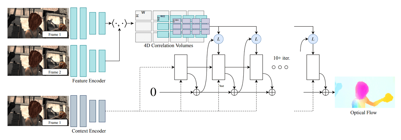 RAFT Architecture
RAFT can be divided into three main parts: Feature Encoder, Context Encoder for feature extraction, Correlation Layer for creating the Correlation Volume between images, and Update Operator for updating and refining the Flow Field from an initial value (Zero) through iterations. Through this three-stage architecture, RAFT computes Optical Flow in the following order:
- Feature Extraction
- Computing Visual Similarity
- Iterative Updates
Feature Extraction
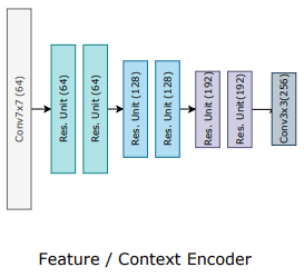 Feature Extractor
Feature extraction plays a critical role in optical flow estimation, as it is responsible for computing visual similarity between two input frames. RAFT employs a feature extractor composed of two sub-networks: Feature Encoder Network (F-Net) and Context Encoder Network (C-Net).
F-Net is a convolutional neural network (CNN) that extracts features from down-sampled images. It computes a feature vector for each pixel of the input frames, generating feature maps for Frame 1 and Frame 2. The feature maps are then used to compute the visual similarity between the two frames, which is a critical step in the optical flow estimation process.
On the other hand, C-Net extracts context features from Frame 1. It is similar in structure to F-Net, but it only extracts features from Frame 1 to capture its contextual information. This feature map is fed to the Update Operator as an input to refine and update the flow field iteratively.
Both F-Net and C-Net are based on a ResNet architecture and produce 256-channel feature maps. By extracting feature maps from both frames and capturing the contextual information, RAFT is able to compute optical flow accurately and robustly.
4D Correlation Layer (Correlation Volume)
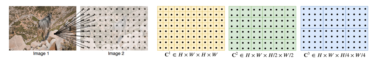 Building Correlation Volumes
The correlation layer, which has been used in optical flow models since FlowNet, is also used in RAFT. Since we have already covered the basic concepts of the correlation layer in the review of FlowNet/FlowNet2.0, we will not cover it in detail here. However, the figure 38 does an excellent job of explaining what it means to create a correlation volume, so I decided to include it. Before delving into the correlation layer of RAFT, if you want to learn more about the correlation layer used in optical flow models in general, please refer the FlowNet and FlowNet 2.0.
In RAFT, there is a slight difference between the timing of generating and using the correlation volume. This can be divided into before and after the iteration process based on the entry point of the Update operator. Let’s take a closer look at this aspect.
4D Correlation Volume Generation - Before Iteration
\[\mathbf{C}(g_\theta (I_1),g_\theta (I_2))\in \mathbb{R}^{H\times W \times H \times W}, \quad\quad C_{ijkl}=\sum_{h}g_\theta (I_1)_{ijh}\cdot g_\theta (I_2)_{klh}\]Unlike conventional correlation, RAFT generates a 4D correlation volume. As shown in the equation above, it stores the results of $Image_{1}(i, j)\cdot Image_{2}(k, l)$. As a result of the equation, a tensor of $H_{1} \times W_{1}$ is created, each with a size of $H_{2} \times W_{2}$. That is, the total size is $H_{1} \times W_{1} \times H_{2} \times W_{2}$.
\[C^k:\begin{bmatrix}H \times W \times \frac{H}{2^k} \times \frac{W}{2^k} \end{bmatrix}\]One special point can be seen in figure 38. With the above equation, we can obtain the result for $C^{1}$. From now on, we generate the Correlation Pyramid by downsampling, using average pooling with kernel sizes of {1, 2, 4, 8}, resulting in $C^{1}, C^{2}, C^{3}, C^{4}$ as the final outputs. The use of average pooling is a good approach to quickly compute coarse correlation.
We now have a deterministic Correlation Pyramid for $Image_{1}$ and $Image_{2}$. Therefore, during the iteration process, we can significantly reduce the overhead by not performing correlation calculations separately.
Correlation Lookup - During Iteration
After entering the Update operator, the precomputed Correlation volume is referenced through the Correlation Lookup process. The Correlation volume is bilinearly sampled around the location corresponding to the current Optical Flow. The 3D Correlation feature is obtained by using the sampled Correlation volume and the Current Optical Flow. Finally, the resulting $(2r+1)^2$ vectors for each Target point are reshaped into a tensor of size $H \times W \times (2r+1)^2$.
Update Operator
RAFT uses a GRU structure to gradually approach a more accurate flow field as it iterates. This can be thought of as stacking layers recursively using CNNs, which has a very similar shape to RNNs (in fact, it is same). Understanding RNN-like architectures has become increasingly important in the computer vision field as transformers continue to invade. However, in this post, we will simply summarize and move on.
 Update operator of RAFT
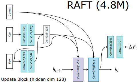
In the figure, three inputs are combined and fed into the ConvGRU, which is the Update operator. The previous hidden state is also added to these inputs to form the final input, and the output is passed through an additional convolutional layer. This process determines the current Flow field, which can be iteratively updated to obtain the final Flow field.
- Inputs
- $x_{t}$: Encoded previous Optical Flow + Encoded Correlation lookup + Output of C-Net
- $h_{t-1}$: Previous hidden state, which is a hidden unit of GRU.
During the iteration process, the Flow field is updated according to the following equation:
\[f_{k+1}=f_{k}+ \bigtriangleup{f_{k}}\]Here, $\bigtriangleup{f_{k}}$ is the Flow field that results from the iteration, and the output is updated from an initial value of 0. This is reasonable since there is no previous frame or any change in the initial state. The paper extensively discusses the iteration process and its considerations. We will explore these points later.
Iteration
In RAFT, there are two main aspects to consider with respect to iterations: training and inference. Let’s take a look at each one.
Training
The training process of RAFT follows a form where the loss becomes more significant as the iteration progresses. Although a straightforward and reliable method is chosen to calculate the error loss with the ground truth, it reflects the features well by comparing all feature maps in the iteration with the ground truth. In this case, if the iteration increases, the weight also increases. The experimental optimal value is shown as $\gamma=0.8$ in the equation below.
\[L=\sum_{i=1}^{N}\gamma ^{i-N}\left\|\mathbf{f}_{gt}-\mathbf{f}_i \right\|_1\]Inference
In inference, there are two methods called Zero Initialization and Warm Start that consider iteration. Zero Initialization sets the initial value of the Flow field to 0, and since it has already been examined, it will not be further discussed. Warm Start is a method proposed to utilize the previous flow, and it is a Forward Projection technique that actually moves and uses it for the next initialization. This is to utilize the previous flow field as a guide in the next iteration, and the following equation is used for this purpose:
\[f_{t}(x+f_{t-1}(x))=f_{t-1}(x)\]Result
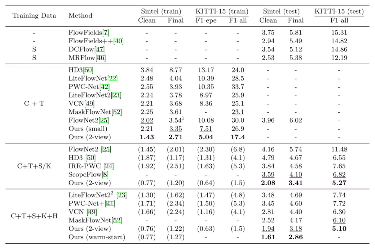 EPE of RAFT
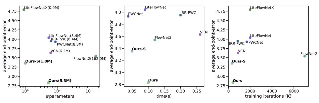 Plots comparing parameter counts, inference time, and training iterations vs. accuracy
Appendix
I was quite pleased with RAFT because it incorporates the method I tried in my graduation thesis. This method was able to reduce the accuracy by around 1%, but it took a long time and had the problem that it was impossible to define the processing time. In particular, the process of creating a correlation volume each time had a large overhead, and I was greatly impressed by the author of RAFT solving this problem. The content is included in section 2.6 Error Correction of the paper, and the image below captures the content.
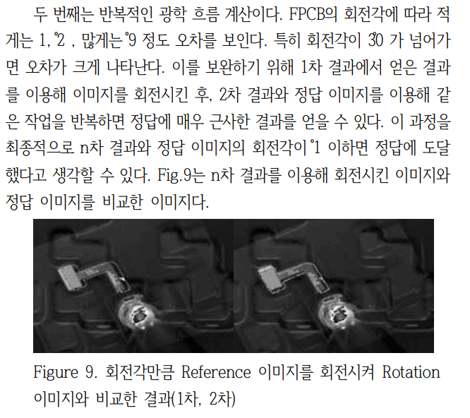 2.6 오차 보정
Leave a comment