
[Optical Flow/11] PWC-Net (CVPR 2018)
This post is written by YoungJ-Baek
You can see the original Korean version at Searching Fundamental
Preface
In previous posts, we covered the first DL-based Optical Flow algorithm, FlowNet, and its improved version, FlowNet2.0. In this chapter, we will discuss PWC-Net, which combines several techniques used in classical Optical Flow algorithms and applies them to a CNN model. PWC-Net can be thought of as an all-in-one solution that incorporates all the popular techniques used in Optical Flow algorithms.
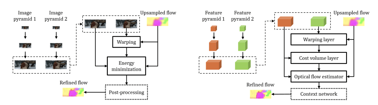 Traditional coarese-to-fine approach vs. PWC-Net
Architecture
The architecture of PWC-Net can be understood by looking at the origin of its name. Net refers to network, and PWC is an acronym for the Optical Flow algorithm techniques applied in this model. The paper suggests that by incorporating these techniques, they have achieved a reduction in model size and an increase in performance. Below are the meanings of PWC:
- (P)yramid Processing (Structure)
- (W)arping Layer (Backward Warping)
- (C)ost Volume Layer (Correlation Layer)
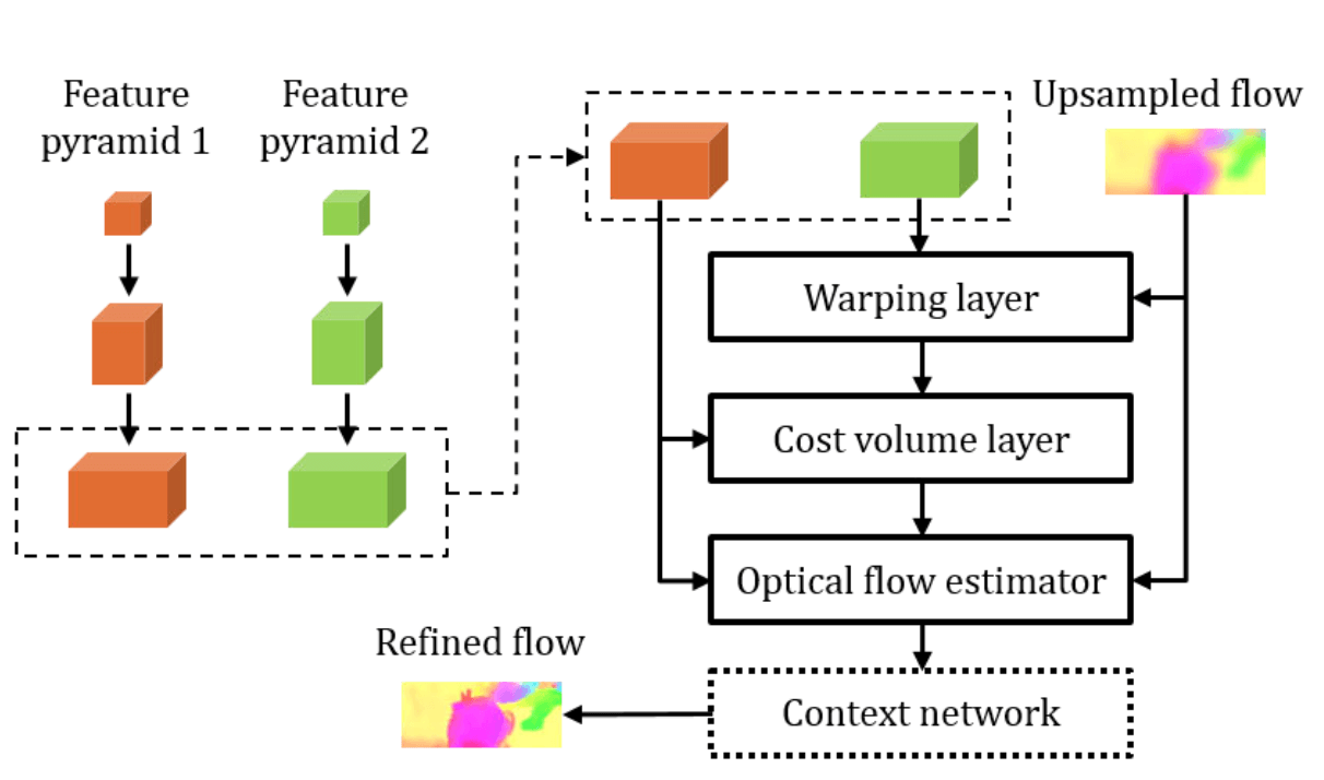 PWC-Net Architecture
As briefly mentioned in the introduction, PWC-Net seems to have been inspired by the approach of classical coarse-to-fine optical flow algorithms. If we focus only on the PWC part of the name, we can understand the meaning of this model more easily. From now on, we will take a closer look at each component of PWC.
Pyramid Structure
Image pyramid is a traditional technique used in the fields of image processing and computer vision. This idea has also been adopted in ML/DL-based optical flow algorithms, and is extensively described in SpyNet [CPVR 2017]. (Since this post does not cover SpyNet, please refer to its reference for more information.)
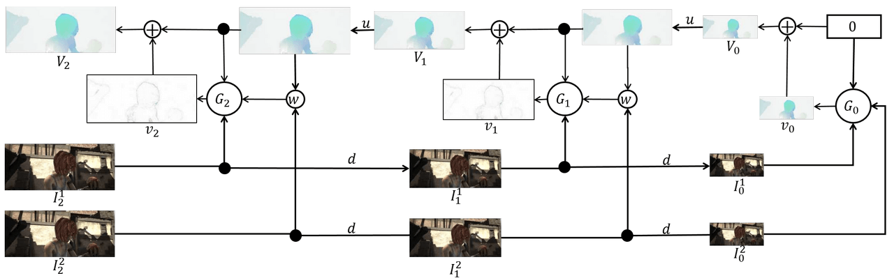 Inference in a 3-Level Pyramid Network
The Pyramid Structure is a structure that obtains Optical Flow by upscaling the down-scaled input image. This helps to compensate for one of the weaknesses of Optical Flow, which is Large Motion Displacement. By securing information about Large Displacement in the Downscale process and securing detail (Small Displacement) in the Upscaling process, it shows strong resistance to large changes.
In PWC-Net, this Pyramid Structure is represented as a Learnable feature pyramid. Unlike the classical method that used raw images as input, feature maps are used as input. Two input images pass through a convolution layer and create an L-level pyramid based on the feature map by downsampling.
Warping Layer (Backward Warping)
Warping refers to the process of adding the up-scaled previous pyramid’s flow to the second image. Optical flow obtained from an operation, not a predicted value, is used to move the actual image. In other words, the motion vector obtained by up-scaling the flow from the previous pyramid is added to $Input \,\, Image_1$. This results in the creation of Groundtruth $Input \,\, Image_2$ and $Input \,\, Image_2’$ through warping. These two may be similar, but they will not be exactly the same, and the smaller the error, the more accurate the operation is.
Why is this process important? If warping is done, learning can be done L times (L-level pyramid structure) through a single training. During the down-scaling → up-scaling process, the error between $Input \,\, Image_2$ and $Input \,\, Image_2’$ can be added as a weight in real-time. (It can be differentiated using bilinear interpolation, and end-to-end operation can be performed.)
In summary, warping improves training efficiency and allows for real-time compensation for geometric distortion by estimating errors in large motion.
Cost Volume Layer (Correlation Layer)
The Cost Volume (Correlation Layer) is a concept proposed in FlowNet [ICCV 2015], which stores matching costs between pixels by performing inner product operations between feature maps. Detailed concepts for this have already been covered in the FlowNet post, so please refer to the post. Here, in order to reduce computational costs, the Cost Volume is computed between feature maps instead of raw images.
\[\mathbf{cv}^l(\mathbf{x_1, x_2})=\frac{1}{N}(\mathbf{c}^l_1(\mathbf{x_1}))^T\mathbf{c}^l_w(\mathbf{x_2})\]Optical Flow Estimator & Context Network
The Optical Flow Estimator and the Context Network both produce Optical Flow as their output. The difference is that the former outputs the Optical Flow prediction for each level of the Pyramid Structure, while the latter outputs the overall result.
- Optical Flow Estimator: Receives $Input \,\, Image_1$, Cost Volume, and Upsampled Flow as inputs to predict Optical Flow for each level of the Pyramid.
- Context Network: Combines the Optical Flow generated at each level of the multi-level pyramid into one (Refined Flow).
Result
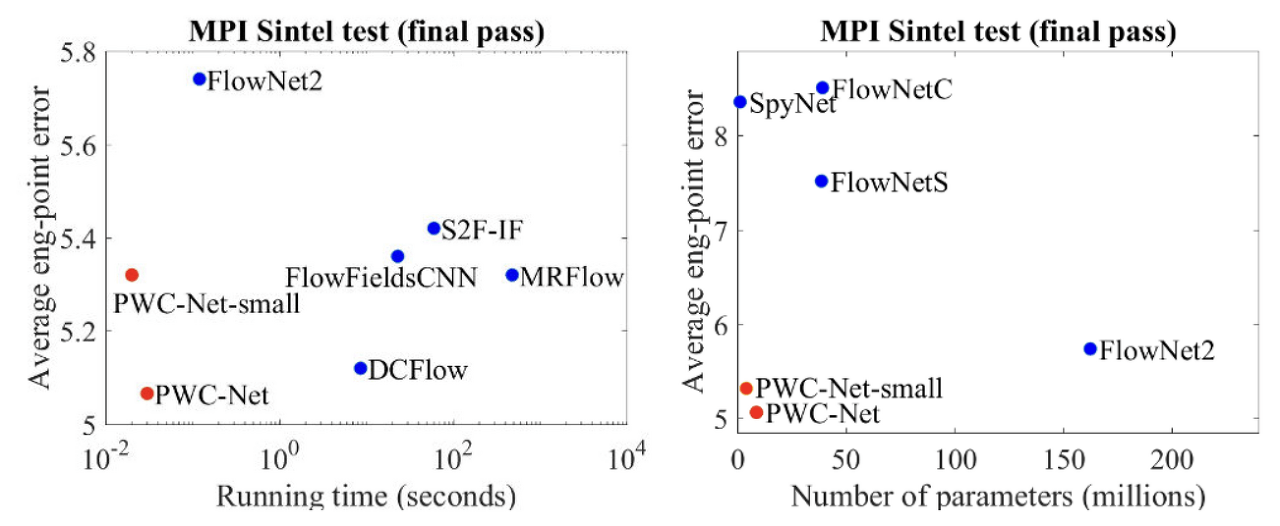 Performance & EPE comparison
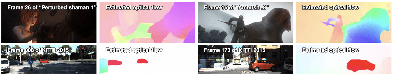 PWC-Net results on Sintel final pass (top) and KITTI 2015 (bottom) test sets
Leave a comment