[Optical Flow/03] Optical Flow Constraint Equation

This post is written by YoungJ-Baek

You can see the original Korean version at Searching Fundamental

Preface

In the previous post, we learned about what Optical Flow is. We also discussed the significant loss of information that occurs when compressing from 3D to 2D. To overcome this problem, Optical Flow makes several assumptions. The coherence concept we covered in the first post reappears here, but with a different name.

Assumptions

In order to calculate the 3D motion from an image compressed into 2D, we need to make assumptions. This must be done within the range that does not distort reality, and it should serve as an important clue to solving the problem.

Brightness is constant

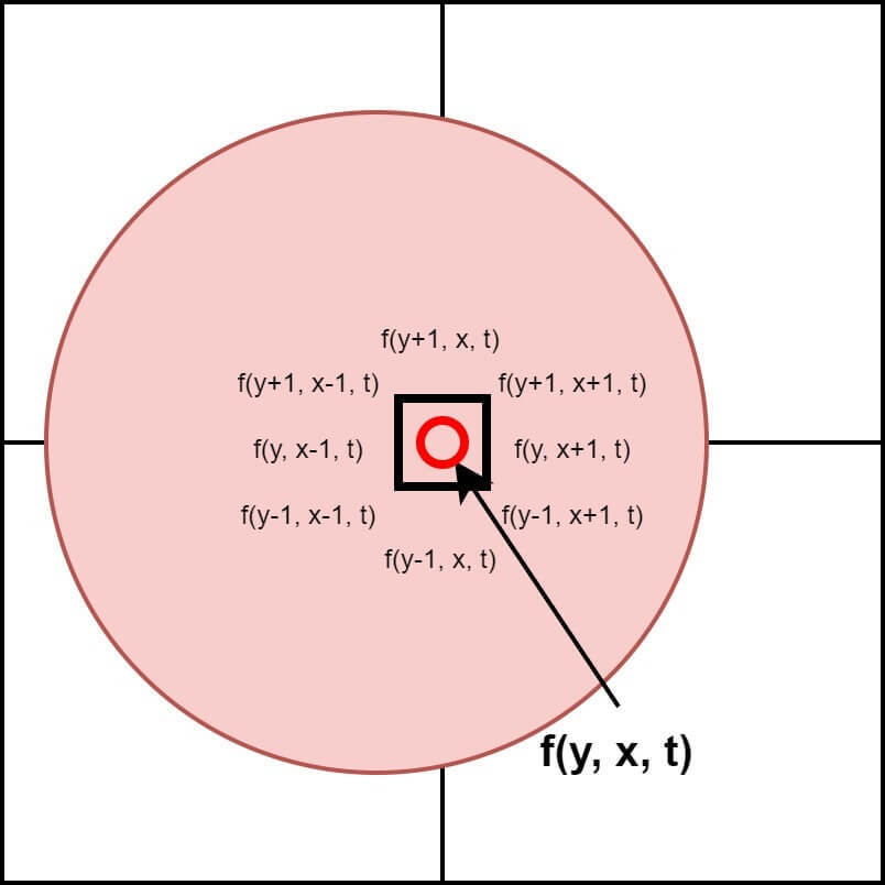Image Coherence

Bright Constancy is an assumption that corresponds to the Image Coherence discussed in the first post. It assumes that in an image, a specific point, that is a pixel, and its neighboring pixels have the same color or brightness. In computer vision, color or brightness are represented by pixel values, so ultimately neighboring pixels have the same value.

However, for this assumption to hold true perfectly, it should be assumed that there are no changes in lighting. Additionally, changes in the angle between the object and the light source should not result in differences in brightness. In reality, it is impossible to create such conditions. To use Optical Flow in the real world, it must follow the laws of the real world. Fortunately, in practice, this assumption cannot be perfectly satisfied, but the errors can be accommodated by using a threshold to accept the degree of error that can be tolerated. Thanks to this, we can use important assumptions to design Optical Flow algorithms.

Motion is small

Time Coherence

Small Motion is the assumption that corresponds to Time Coherence discussed in the first post. Large changes require small changes to precede them. The Optical Flow we are dealing with assumes small changes because it deals with changes between two consecutive frames.

In two consecutive frames, the same pixel of an object has the same brightness/color (i.e., the pixel values are the same or similar).

These two assumptions can be expressed as above, and they are the most important assumptions for calculating Optical Flow, so it is important to keep them in mind. In fact, if you think about it for a moment, it is a very obvious proposition. However, as with many assumptions in computer vision, it is a process of assuming the obvious to solve problems.

Optical Flow Constraint

How to estimate pixel motion from one image to another?

At time $t$, let’s call the intensity of a point $(y, x)$ in the image as $I(y, x, t)$, and its value at $t+1(=t+dt)$ as $I(y+dy, x+dx, t+dt)$. Applying the first assumption, Brightness Constancy, we can derive the A equation below.

\[I(y,x,t)=I(y+dy,x+dx,t+dt)\Rightarrow A\]

If we apply Taylor series (expansion) to the right-hand side of the equation, we get the B equation as follows.

\[I(y+dy,x+dx,t+dt)=I(y,x,t)+\frac{\partial I}{\partial y}dy+\frac{\partial I}{\partial x}dx+\frac{\partial I}{\partial t}dt+\cdots \Rightarrow B\]

The omitted terms are second-order or higher-order terms. As these terms have a significantly smaller impact than the first-order term when $dy$ and $dx$ are sufficiently small due to the second assumption, Small Motion, and the time interval between two consecutive frames, $dt$, is sufficiently small, we can omit them completely.

However, it is not possible to define the exact value of a sufficiently small time interval, $dt$. It is a value that allows $dy$ and $dx$ to remain sufficiently small. Typically, if the movement of an object can be captured within a few pixels, it is considered a sufficiently small value. Therefore, what is important is not just the time interval, but also the amount of movement during that time interval.

Returning to the main topic, substituting the simplified B equation obtained under the assumption of a sufficiently small time interval into the A equation yields the following equation.

\[I(y,x,t)=I(y,x,t)+\frac{\partial I}{\partial y}dy+\frac{\partial I}{\partial x}dx+\frac{\partial I}{\partial t}dt+\cdots \Rightarrow B\,in\,A\]

If we simplify the previous equation a little more, we can get the desired form. The following equation finally allows us to focus on the change. While there is a method to derive this equation directly from the Taylor expansion through Brightness Constancy, we have shown the step-by-step derivation from the beginning for better understanding.

\[\frac{\partial I}{\partial y}dy+\frac{\partial I}{\partial x}dx+\frac{\partial I}{\partial t}dt=0\]

If we divide both sides of the equation by $dt$, it can be expressed as follows.

\[\frac{\partial I}{\partial y}\frac{\mathrm{d} y}{\mathrm{d} t}+\frac{\partial I}{\partial x}\frac{\mathrm{d} x}{\mathrm{d} t}+\frac{\partial I}{\partial t}=0,\quad I_yv+I_xuI_t=0\]

The second equation is a simplified version of the first equation, where each term has its own meaning. This equation is called the Optical Flow Constraint Equation, OFC for short, and sometimes also referred to as the Gradient Constraint Equation. Most Gradient-based Optical Flow algorithms are derived from this equation. However, this equation alone cannot calculate Optical Flow or Motion Vectors, and the reason for this is as follows.

Apperture Problem

Let’s take a closer look at the OFC. Before examining the meanings of each term, let’s separate them into variables and constants. The terms expressed by partial derivatives are constants that are determined dependently if the position and value of the pixel for which Optical Flow is to be measured are fixed. Therefore, the partial derivatives are constants, and the remaining terms expressed by derivatives can be viewed as variables. If you’ve followed this perfectly so far, you can discover a big problem. Is something weird? Isn’t the equation weird? Brilliant! That’s a great question. The above equation is weird. No, to be precise, it is insufficient. Let’s first understand the meanings of the OFC terms.

Constants

\[\left ( \frac{\partial I}{\partial y},\frac{\partial I}{\partial x}\right )\Rightarrow Gradient\,\, Vector,\quad \frac{\partial I}{\partial t}=I(x,y,t+1)-I(x,y,t)\]

Variables

\[\left ( \frac{\mathrm{d} y}{\mathrm{d} t},\frac{\mathrm{d} x}{\mathrm{d} t} \right )\Rightarrow Motion\,\,Vector,\quad\frac{\mathrm{d} y}{\mathrm{d} t}=v,\quad\frac{\mathrm{d} x}{\mathrm{d} t}=u\]

The three vectors that make up the constant term are values measured from the image, and (v, u) must be calculated using these values. Here, a strange point is discovered. There is only one equation, but there are two unknowns to be solved… The equation is insufficient. In other words, the Optical Flow Constraint Equation cannot uniquely determine the Motion Vector. This means that without other assumptions, it is impossible to determine the motion at a single point. This problem is known by various names such as the “pinhole problem” or “aperture problem.”

Conclusion

In this post, we looked at the important assumptions and equations, including the Optical Flow Constraint Equation (OFC), for calculating Optical Flow. You may have felt frustrated after following along diligently but realizing that we can’t determine the Motion Vector with just one equation. However, as an Algorithm Engineer, if the equation is incomplete, we can add additional assumptions to fill it out. In fact, in the next post, we will explore the more commonly known Lucas-Kanade and Horn-Shunck algorithms, which add conditions to find solutions to equations and determine the Motion Vector. Let’s first take a closer look at the Lucas-Kanade algorithm.

Reference