[Optical Flow/04] Lucas-Kanade Algorithm, Part I

This post is written by YoungJ-Baek

You can see the original Korean version at Searching Fundamental

Preface

The Optical Flow Constraint Equation (OFC) we derived earlier is insufficient to actually compute the Optical Flow. With two unknowns and only one equation, we cannot determine a solution. Therefore, we need to add assumptions, and the first method we will discuss is the Lucas-Kanade method. We will present the added assumption, the computation of Optical Flow, and the advantages and disadvantages in that order.

Assumptions

The assumption added in the Lucas-Kanade Method highlights the characteristics of the algorithm well. The Optical Flow of the $n \times n$ window $N(y, x)$ created around the pixel $(y, x)$ are all the same. That is, the pixels inside the window move in the same direction, and therefore have the same Motion Vector values. This indicates that the algorithm finds the solution of the Optical Flow problem using a local approach. With the addition of the new assumption, the Lucas-Kanade Algorithm now has a total of three assumptions, in addition to the two existing ones:

• Brightness is constant
• Motion is Small
• Flow is essentially constant in a local neighborhood of the pixel

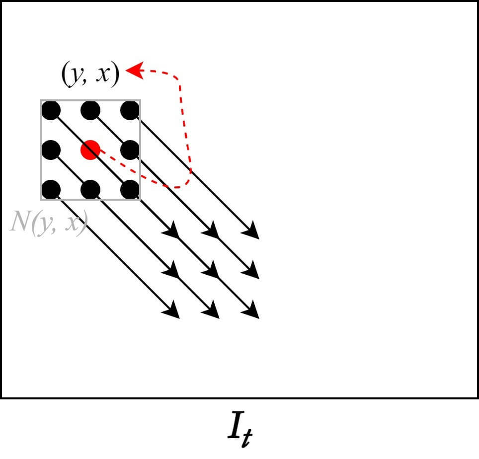Additional Assumption for Lucas-Kanade Algorithm

The OFC can be modified with the addition of this new assumption. The window size in this case is the number of pixels included in $N(y, x)$. The modified OFC with the new assumption is as follows.

\[\frac{\partial I(y_{i},x_{i})}{\partial y}v+\frac{\partial I(y_{i},x_{i})}{\partial x}u+\frac{\partial I(y_{i},x_i)}{\partial t}=0,{\quad}(y_i,x_i)\in N(y,x)\]

To transform the above equation into a matrix form, we can expand it as follows. Let $p$ be the center point of the window, and let $q$ be the neighboring pixels of $p$, although they do not appear in the following equation.

\[I_x(q_1)V_x+I_y(q_1)V_y=-I_t(q_1)\] \[I_x(q_2)V_x+I_y(q_2)V_y=-I_t(q_2)\] \[\vdots\] \[I_x(q_n)V_x+I_y(q_n)V_y=-I_t(q_n)\]

Surprisingly, unlike the previous OFC that was insufficient with 2 unknowns and 1 equation, this time the equations overflow. There are $n$ equations depending on the Window Size, so there is no problem in determining the Optical Flow. Now let’s convert the above equation into matrix calculation form of $Av = b$.

\[A=\begin{bmatrix} I_x(q_1) & I_y(q_1) \\ I_x(q_2) & I_y(q_2) \\ \vdots & \vdots \\ I_x(q_n) & I_y(q_n) \\ \end{bmatrix},\quad v=\begin{bmatrix} V_x \\V_y \end{bmatrix},\quad b=\begin{bmatrix} -I_t(q_1)\\ -I_t(q_2)\\ \vdots\\ -I_t(q_n)\\ \end{bmatrix}\]

After converting to matrix form, it is more intuitive that there are too many equations compared to the required number. To reduce the number of equations to the necessary minimum, we can use the Least Squares Principle. We can obtain the Motion Vector by transforming the equation into a form that is a function of $v$, as shown below.

\[A^{T}Av=A^Tb \quad \Rightarrow \quad v=(A^TA)^{-1}A^Tb\] \[\begin{bmatrix} V_x \\V_y \end{bmatrix}=\begin{bmatrix} \sum _iI_x(q_i)^2&\sum _iI_x(q_i)I_y(q_i) \\ \sum _iI_y(q_i)I_x(q_i)& \sum _iIy(q_i)^2 \\ \end{bmatrix}^{-1}\begin{bmatrix} -\sum _iI_x(q_i)I_t(q_i) \\ -\sum _iI_y(q_i)I_t(q_i) \end{bmatrix}\]

Pros and Cons

Finally, we learned a way to calculate Optical Flow. However, the Lucas-Kanade Method is just one of the methods to calculate Optical Flow, as we can create various algorithms by adding different assumptions to the basic OFC. Each method has its own advantages and disadvantages, so it is important to choose the algorithm that is suitable for the situation. So what are the pros and cons of Lucas-Kanade? If you have some experience in Computer Vision, you may immediately think of the answer. The result is highly dependent on the Window Size! If the Window Size is large, the operation will be fast but inaccurate, and vice versa. That’s right. The rest are pros and cons from an Optical Flow perspective, so you don’t have to feel overwhelmed if you don’t immediately understand them. It’s natural to not know everything.

• Pros
  • It belongs to Sparse Optical Flow and uses points with prominent features such as edges, resulting in low computation.
• Cons
  • The Window Size is generally small, so it cannot calculate movements larger than the window.
  • Since it calculates Optical Flow based on a specific point, the accuracy is lower than that of Dense Optical Flow, which calculates globally.

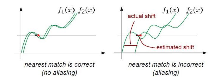
The part that may be difficult to understand in the cons is probably when there are movements larger than the window. Since it is based on value tracking, Isn’t it okay even if the movement is large? The problem is that window-based algorithms do not consider outside the window. Therefore, aliasing occurs in this case, resulting in distortion as shown below.

Aliasing by Big Motion in Lucas-Kanade Algorithm

Conclusion

In this post, we learned how to calculate Optical Flow using the Lucas-Kanade Algorithm and its additional assumptions. We also learned that LK is not a perfect method, as it has its own advantages and disadvantages. Algorithm engineers continue to work on improving this method when problems arise. There are numerous ideas to improve LK, including using weights that are common in window-based algorithms to improve accuracy and proposed methods to deal with Big Motion, which we will discuss in the next post. Additionally, we will mention the persistent problems of Sparse Optical Flow that were not covered in this post. Through this process, we will experience the extension of the concepts previously mentioned.

Reference