
[Optical Flow/09] FlowNet (ICCV 2015)
This post is written by YoungJ-Baek
You can see the original Korean version at Searching Fundamental
Preface
In the previous post, we looked at Handcrafted Optical Flow techniques. From now on, we will cover research on obtaining Optical Flow through Deep Learning. It all started with FlowNet, which was presented at ICCV 2015. Before FlowNet, there was a lack of research on hardware and Deep Learning, and the most important point was the lack of Optical Flow Groundtruth datasets required for learning. In this post, we will examine how FlowNet overcame these limitations.
FlowNet is an algorithm that uses supervised learning to estimate optical flow. It overcame the limitation of the lack of optical flow ground truth data for supervised learning by using its own method. This approach made a significant contribution to optical flow research, and we will cover it in the Dataset section.
FlowNet is an end-to-end CNN-based learning method. Since optical flow takes two images as input, it introduced a correlation layer to perform pixel-level localization for end-to-end learning.
Traditional handcrafted optical flow estimation methods such as Lucas-Kanade and Horn-Schunck manually set the algorithm’s parameters without separate training. Therefore, performance differences may occur depending on the engineer’s skill and understanding. However, FlowNet, which uses deep learning techniques, can minimize human intervention and solve such problems.
Dataset
Generating ground truth for optical flow estimation is a challenging task, as existing algorithms may have bias or inaccuracies. However, manually creating data for training may also result in an unsuitable format for machine learning. To address this issue, FlowNet created a synthetic dataset called Flying Chairs, which combines 3D chair images with Flicker DB. This allows for the creation of training data that is difficult to obtain in real life, while avoiding the limitations of manual data creation.
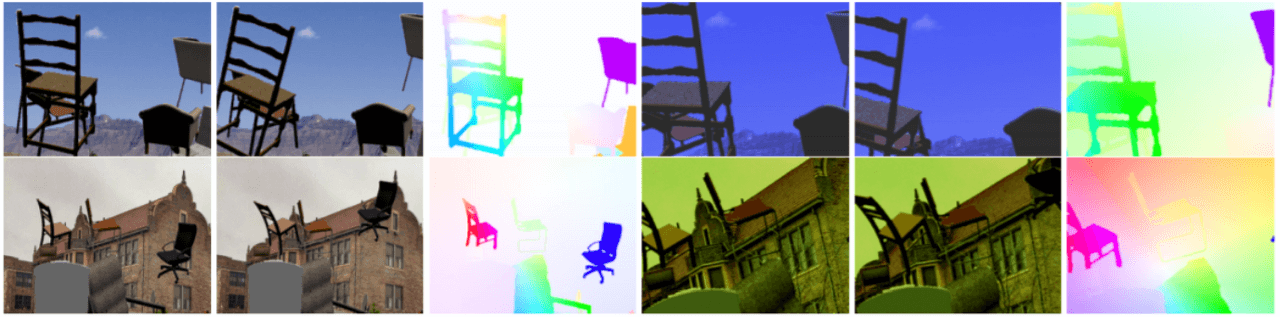 Flying Chairs Dataset
The Flying Chairs dataset proposed in FlowNet was not just an idea but actually succeeded in estimating optical flow. This demonstrated that a network trained on synthetic images can be applied to real-world images. Subsequently, many synthetic datasets, including Flying Chairs, have been widely used for learning in other optical flow research where real data is scarce.
Concept
To obtain optical flow between two frames, it inevitably requires two inputs. To learn in an end-to-end format with two input values, FlowNet proposes two methods. First, following figure is a basic concept image of FlowNet.
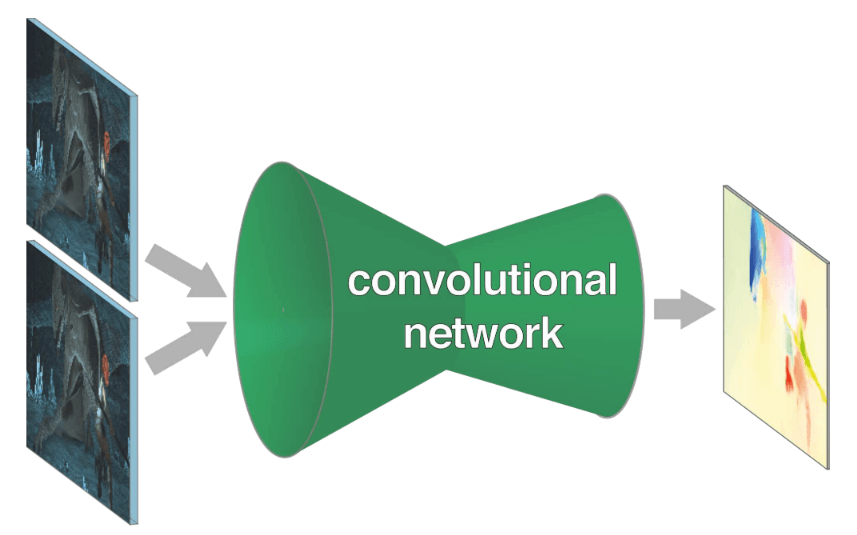 Concept image of FlowNet
The Optical Flow is computed by training a CNN architecture in an End-to-End manner. Depending on the network architecture, there are two models: the FlowNetS, which is a generic architecture, and the FlowNetC, which uses the correlation of feature maps between the two input images. S and C stand for Simple and Corr (Correlation), respectively.
In addition, to achieve practical learning considering the computational complexity, pooling layers are used. This has the effect of combining information from a wide area, which I think is similar to the Coarse-to-Fine technique used in traditional Optical Flow methods.
Like the Coarse-to-Fine technique, a process of restoring the reduced resolution is necessary. In FlowNet, this process is performed by the Refinement layer, which acquires a pixel-wise Flow Map with the same resolution as the input images, resulting in a CNN-based End-to-End model.
Architecture
FlowNet proposes two architectures, FlowNetSimple (FlowNetS) and FlowNetCorr (FlowNetC), as shown in following figure.
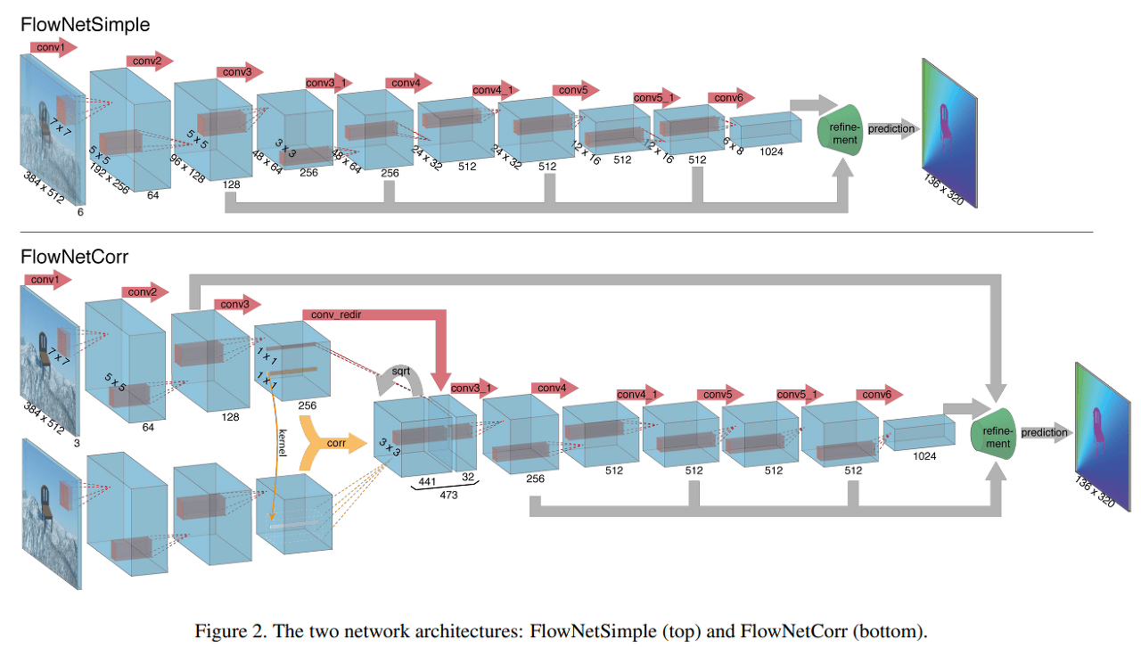 FlowNet Architecture
FlowNetSimple
FlowNetSimple is a simpler network that concatenates two input images required for optical flow calculation into a single input channel of size 6. The subsequent network structure follows the traditional CNN architecture, and it is trained using supervised learning to enable the network to determine the optical flow extraction method on its own.
FlowNetCorr
FlowNetCorr has a more complex structure compared to FlowNetSimple. The number of input channels is reduced to 3, indicating that there is no concatenation process. Instead, the input is divided into two input streams for the two input images. The input streams are identical in structure and each stream extracts the feature maps of the corresponding input image. The Correlation layer is used to merge these feature maps into a single representation. The authors of the paper refer to this feature map as the meaningful representations of the two images.
The question arises as to how the Correlation layer merges feature maps obtained through feature extraction rather than images. We will explore this in detail in the following post.
Correlation and Refinement Layer
FlowNet mostly follows a conventional CNN architecture, so it is not difficult to understand. However, the Correlation layer requires additional explanation. We will also provide an explanation of the Refinement layer, which is not usually seen in conventional CNN architectures.
Correlation layer
The paper expresses the Correlation process using the following equation:
\[c(\mathbf{x_{1}}, \mathbf{x_2}))=\sum_{\mathbf{o}\in [-k,k]\times[-k,k]}\left<\mathbf{f_1(x_1+o),f_2(x_2+o)} \right>\]First, we need to define $d, D, k, and K$ for correlation. This process is complex to express in words, so we will omit it and provide a link to the paper in the references for your reference. After defining the region, if we look at the correlation operation at the vector unit level, we can see that it can be viewed as the dot product between the vector at position $\mathbf{x_1}$ and the vector at position $\mathbf{x_2}$. Simply put, this is the process of stacking the resulting values obtained by taking the dot product of each element of the pre-defined patch and then summing them along the channel axis.
\[(w \times h \times D^2)\]The output of the Correlation layer is a rectangular parallelepiped of the size of the above value. Following figure is an example illustration to help understand the Correlation layer.
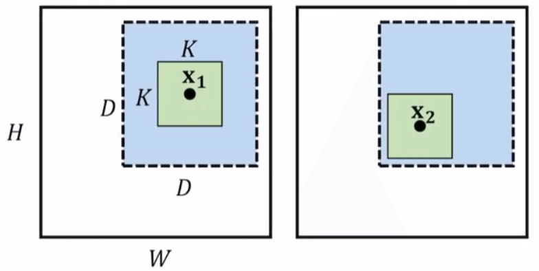 Correlation layer Example
Refinement layer
The refinement layer is the final layer in FlowNet. Both FlowNetS and FlowNetC have refinement layers. First, let’s examine the structure through following figure.
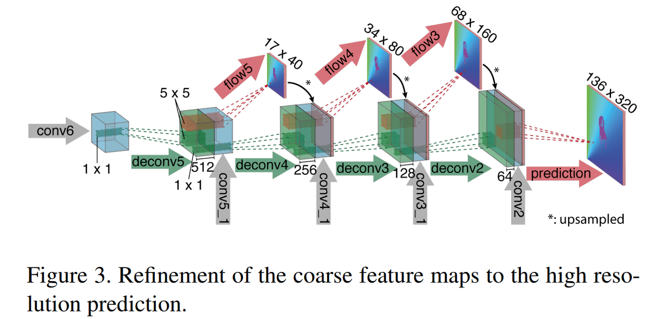 Refinement layer
As shown in the figure, the Refinement layer is a structure that repeats Upsampling and Convolution. It also uses a concatenation method that concatenates the layers calculated in the front, such as conv5_1 and conv4_1, in between.
In addition, Flow Maps for intermediate results such as flow5 and flow4 are extracted, and the loss is calculated by comparing them with the Downsampling version of the Groundtruth image. Optical Flow often uses the EPE (End Point Error) Loss, which is the L2 Loss between the Estimated and Groundtruth values.
Contribution
From the content written so far, FlowNet seemed like an innovative technique that would bring an end to handcrafted approaches. However, surprisingly, the performance of FlowNet did not turn out as good as expected.
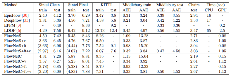 Average EPE Loss
FlowNet has sufficient contributions beyond being the end of handcrafted techniques, even though its performance is not as good as Epicflow, which is considered the pinnacle of handcrafted techniques, in terms of EPE. It has been confirmed that synthetic images can be used for training that is applicable to real-world scenarios. Additionally, the Flying Chairs Dataset, which is essential for DL-based Optical Flow research, was created. The calculation speed of Optical Flow, which was only possible with CPUs, was greatly improved by bringing it into the GPU domain.
Furthermore, with the release of FlowNet2.0 at CVPR 2017, it proved the significance of their direction for improving the performance of FlowNet. It is a meaningful paper that I was responsible for in my graduation research. FlowNet2.0 can be said to inherit everything from FlowNet. Therefore, a high level of understanding of FlowNet is essential.
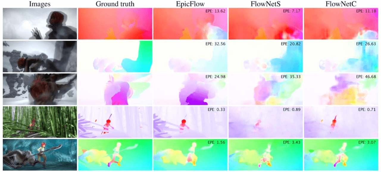 Examples of Optical Flow prediction on the Sintel dataset
Leave a comment