
[Optical Flow/06] EpicFlow (CVPR 2015)
This post is written by YoungJ-Baek
You can see the original Korean version at Searching Fundamental
Preface
In the previous post, we talked about improving the accuracy of the Lucas-Kanade Algorithm through weighting and proposed methods to address Big Motion. We have so far discussed the most representative Handcrafted method, Lucas-Kanade, and in this post, we will discuss EpicFlow, which is considered the essence of Handcrafted techniques (my personal opinion). This will be the last time we mention Handcrafted techniques (Horn-Schunck, etc. will be covered if I have time). The reason for covering EpicFlow last is because it is often cited as a benchmark for comparison with Deep Learning-based techniques that will be introduced in the future.
Architecture
EpicFlow is a paper presented at CVPR2015. It added something to the Coarse-to-Fine technique used in Lucas-Kanade and similar ideas to improve performance. You can easily understand this idea by looking at the picture.
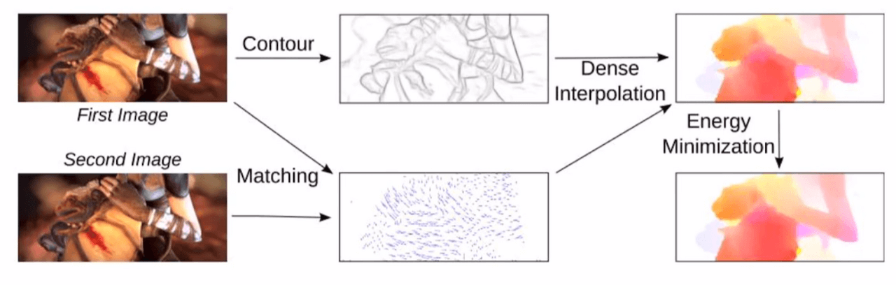 Architecture of EpicFlow
EpicFlow goes through three major steps to obtain a Flow Map. First, it uses a matching algorithm to obtain a matching sparse set between two images. The algorithm used for this step is the one that has the best performance (state-of-the-art). Then, it obtains a precise Flow Map through sparse-to-dense interpolation that corresponds to Coarse-to-Fine. Finally, it uses energy minimization to obtain the final Optical Flow.
The above explanation contains too many proper nouns, and the description is somewhat unfriendly, to the extent that it is easier to understand the idea through the figure. Therefore, I will explain it step by step. Of course, this post is not intended to master EpicFlow. On the contrary, it is closer to understanding the concept of EpicFlow, which is the essence of Handcrafted techniques and a counterpart to Deep Learning techniques in the future. Therefore, I will not provide too detailed an explanation, so please understand.
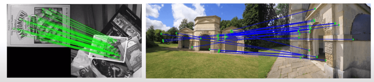
Sparse set of Matches
The first step of EpicFlow is to extract matching pairs between two frames. As mentioned, any state of the art matching algorithm can be used. In experiments, the Deep Matching and Subset of an estimated nearest-neighbor field methods were used. Obtaining matching pairs means matching features between the two images.
Feature descriptor is an example of a matching algorithm, which matches characteristic points between two images with different viewpoints or affine transformations. In other words, it finds the same points in two different images, and it extracts sparse matching pairs through characteristic points such as edges, rather than matching all pixels. For more detailed information on this, I recommend referring to the blog link in the references.
 Feature Descriptor
Interpolation Method
The second step of EpicFlow is to estimate a dense Flow Map through an interpolation process using the matching pairs obtained in the first step. EpicFlow proposes two methods for this:
- Nadaraya-Watson (NW) Estimation
- Locally-weighted Affine (LA) Estimation
In addition, the number of matching pairs used in the interpolation is limited by using local interpolation and only considering the K-nearest neighbors. This improves the computational speed.
Finally, the interpolation results are refined using Energy Minimization to obtain a final Optical Flow with sharper edge points. However, this post will not cover Energy Minimization in detail (it may be covered later along with the Horn-Schunk algorithm if I have time).
Edge-preserving Distance
Now that most of the EpicFlow architecture have been addressed, the remaining one is the Edge Map obtained as a result of contouring. Why is the Edge Map used in EpicFlow? As we learned in previous post, the Coarse-to-Fine technique was used to compensate for the Lucas-Kanade Algorithm’s vulnerability to Large Displacement. However, this method also had an Error Propagation problem, where errors from coarser levels propagate to higher levels.
Sparse-to-Dense Interpolation addressed this issue by utilizing only some of the matching results. However, this process causes a significant loss of information, and selecting sparse feature points is important to achieve a uniform result or an expected value. The Edge Map was proposed here, as the boundaries of new motions are typically observed at the edges of the image. Therefore, EpicFlow preserves the motion boundaries, namely the Edge Map, to calculate Optical Flow.
When using the typical Euclidean Distance, the Flow Map is significantly affected by the surrounding background in the Edge region, causing problems with the result being distorted during interpolation. Therefore, the Geodesic Distance (Edge-aware Distance) is utilized. Geodesic Distance is computationally intensive, so it takes a long time. Therefore, an Approximation is used, but we will not cover it in this post. Instead, let’s learn about the difference between Geodesic Distance and Euclidean Distance in a figure as follows.
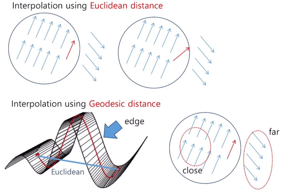 Euclidean distance VS Geodesic distance
Conclusion
Next, we will cover FlowNet, which began measuring optical flow using deep learning. It was a more interesting paper that was released in the same year as EpicFlow, and FlowNet 2.0, which improved performance, was also used for my research topic. However, before we touch deep learning methods, we will gonna touch two basic knowledge of current Optical Flow research. First one is about flow map, which is used for representing the result vectors. Second one is the dataset for Optical Flow in deep learning.
Leave a comment